Tokenomics, behind the scenes

Everything we do at umans.ai comes back to one question: how do we get the highest-value automated work at the lowest cost?

That question splits in two. What does a token cost to produce? And how much useful work does that token perform? The second question is why we serve a short lineup of frontier models and change it carefully: a $0.05-per-million token from a weak model is not cheaper than a $0.50 token from a model that finishes the job in one attempt.

This article is about the first question: what does a token cost to produce? It is tempting to treat it as a hardware question. Put the model on a good GPU, check the hourly rate, divide. Serving models for a living has taught us otherwise:

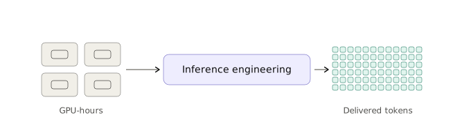
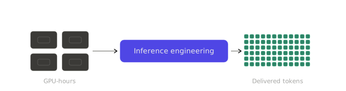
The cost of a GPU does not determine the cost of a token. The whole system that turns GPU time into useful, reliably delivered tokens does.

That system is what the rest of this article walks through.

1. Same model, radically different economics

Here is the observation that motivates everything else: put the exact same model on GPUs, and its token production cost can vary by multiples depending on how you serve it.

Take Kimi K3, one of the frontier models we serve. Different serving setups give the same model very different profiles, something we saw in our own experiments early on, and something you can check in clean public data. Here it is in SemiAnalysis’s InferenceX measurements: one B300 node against a pair of B200 nodes, same agentic workload:

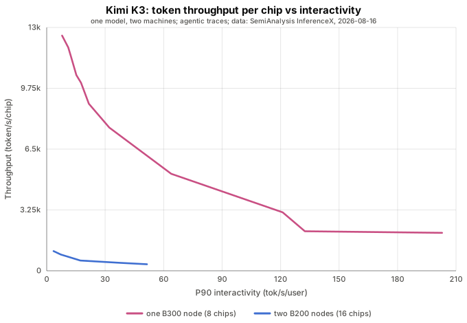
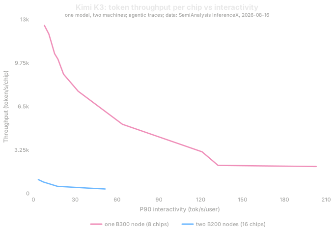
Same weights, same traces, and the per-chip delivery differs by roughly an order of magnitude depending on the machine and how it is driven. How you serve is an economic decision.

DeepSeek published the same effect from their own fleet, on DeepSeek V4 Flash. In their DSpark paper, they shared serving measurements for two generations of their stack: an earlier configuration called MTP, then DSpark, which delivers tokens 57% to 78% faster to each user at the same fleet throughput. Same weights, same fleet, very different economics.

Then we ran the same model through our own serving stack. This is what we measured, first in our lab and then in production:

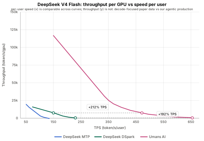
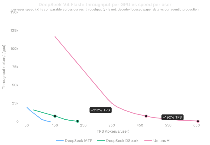
Three curves, one model: blue and green are DeepSeek’s two generations of serving, pink is ours on B200 GPUs. Speeds compare directly: the horizontal axis means the same thing on every curve. Heights measure different workloads, their decode workload against our agentic production, and the next section shows how to read both.

2. There is no single throughput number. There is a frontier.

Two quantities compete inside every serving system:

Production throughput, tokens per second per GPU: what the factory ships.

Interactivity, tokens per second per user: what one person feels.

If we only cared about factory throughput, we would batch aggressively and let every user wait. If we only cared about one user’s speed, we would dedicate enormous capacity to a single request and destroy the economics. So neither claim you see in marketing, “we do 500 TPS” or “we do 100k tokens per second per GPU”, means much by itself. Each is one end of a trade pretending to be the whole story.

The interesting object is the curve between them: for every level of interactivity we promise a user, how many total tokens can the same GPU produce? That is why DeepSeek’s paper talks about shifting a frontier rather than quoting one number, and it is what the chart in section 1 actually shows.

Two things about reading this chart honestly.

Per-user speed is directly comparable, and it is where we live. Since the day the weights were released, nobody has served this model faster: the paper’s own frontier ends near 230 tokens per second per user, public provider tracking tops out well below 300, and our production p50 is 367, with single sessions beyond 590. (Some lab setups have crossed 850. Fun, but not what we optimize for.)

Throughput per GPU is not directly comparable, and the reason is the insight of this article. DSpark was measured on a decode-focused dataset: requests that mostly generate. Our curve is measured on production agentic sessions, trillions of tokens of them every month, and in that real agentic world the work has a different shape: an agent rereads its whole growing workspace before every step, then writes a few hundred tokens. In our production, an average request carries about 134,000 tokens of context for some 800 tokens of output, and 96.8% of that context is served from cache. Serving that shape well is mostly a prefill and cache problem, which is where most of our engineering actually goes, and it is why our axis counts delivered tokens: for automated work, delivered tokens is the number that becomes value and cost. This is us optimizing the question we opened with.

3. Turning the frontier into dollars

A point on the frontier becomes a price with one line of arithmetic, borrowed from NVIDIA’s piece on AI factory economics:

Cost per million tokens = (GPU cost per hour) / (tokens per GPU per second × 3,600) × 1,000,000

To get a feel for it: a GPU renting for $4 an hour that delivers 1,000 tokens per second produces tokens at about $1.11 per million. Make the same GPU deliver 10,000, and the cost drops to 11 cents. Same rent, ten times cheaper tokens.

Now watch it happen to the Kimi chart from section 1. InferenceX prices those same runs with its public TCO model, at $2.60 per chip-hour for the B200s and $3.00 for the B300:

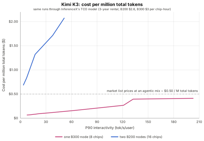
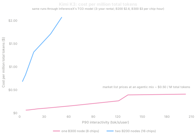
On the B300 node, a million total tokens costs about six cents at the capacity end and about forty cents at 200 tokens per second per user. On the two B200 nodes, the same million costs seventy cents to two dollars, at much lower speeds. The dashed line is what the market’s list prices for this model come to at an agentic token mix, around fifty cents per million total tokens: one of these machines serves it profitably, the other cannot.

Two labels on this chart, then we move on. It prices compute alone, on minimal serving configurations without production redundancy or traffic headroom.

That is intentional: compute alone is the right lens for reasoning about efficiency, and the one NVIDIA’s method uses. A production token also carries redundancy, traffic headroom and the availability you promise, overhead that moves with your SLO; section 5 prices that in.

4. So what actually moves the curve?

Everything above treats the frontier as given. It is not. Every layer of the system pushes it, and each layer is best understood as an economic lever rather than an architecture diagram.

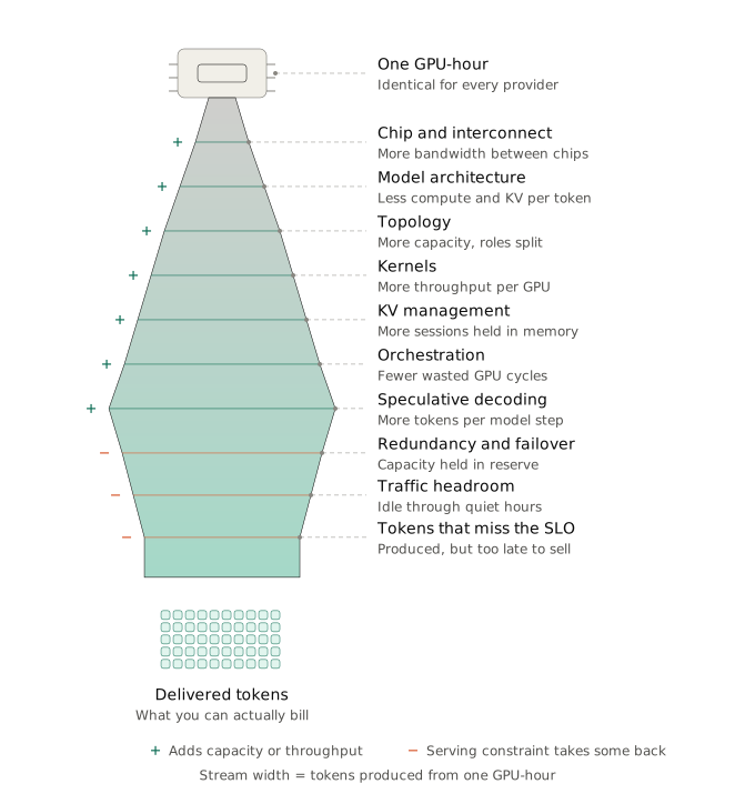
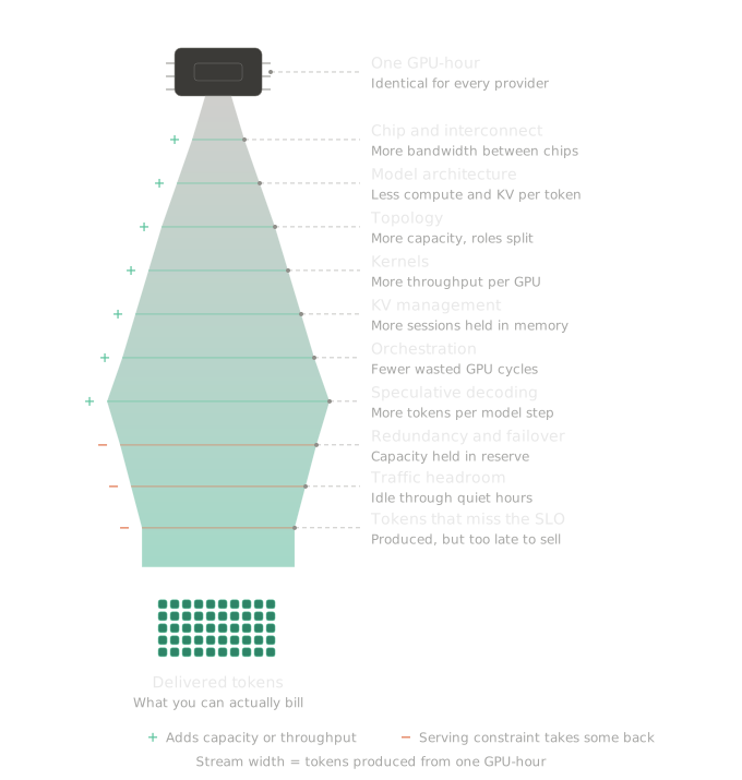
The widening half of that stream is this section. The narrowing at the end is the next one.

The model itself

The model decides how hard the problem is before any serving cleverness begins, along three dimensions. Compute: how much work does one token require? Capacity: how much GPU memory does each session consume, through weights and through the KV state that grows with context? Maturity: is the checkpoint stable enough to deserve serving investment at all? We learned that last one the honest way, serving a preview checkpoint of V4 Pro whose weights were about to be replaced.

DeepSeek V4 shows how directly architecture becomes economics: its compressed attention was designed to cut long-context work and KV footprint, and the technical report measures the V4 architecture at a million tokens of context running at 27% of the single-token FLOPs and 10% of the KV cache of the previous generation. Less compute per token and less memory per session is, quite literally, the curve moving before a single serving decision has been made.

Topology, and the wires between chips

A model has to live somewhere physical, and the choices read like housing decisions: where do the weights live, where does prefill happen, where does decode happen, and what communication do we pay for between them? The building blocks look like this:

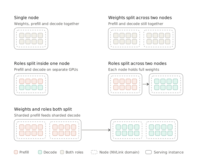
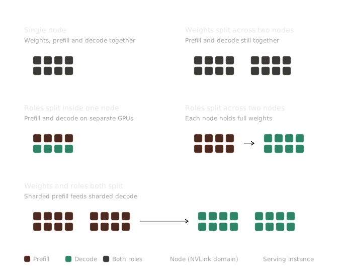
Each block trades the same four things.

Memory. The weights have to fit somewhere, and every live session adds its KV state on top. Splitting the weights across more GPUs buys room for a bigger model and more concurrent sessions.

Communication. The moment you split anything, GPUs have to talk, and the wires set the price. Inside a node, NVLink moves a session’s state in milliseconds and the split feels free. Across nodes you are on a network, and its protocol decides whether the same split is a win or a tax.

Interference. When prefill and decode share the same GPUs, a heavy incoming prompt stalls everyone’s token stream. Splitting the roles removes that, at the cost of the communication above.

Simplicity. One node with everything together is the easiest system to run, and easy is worth real money in operations. You climb the ladder only when the workload pays for the climb.

And the floor plan is only the first cut. Inside each block sit further, orthogonal splits: tensor parallelism (TP), pipeline parallelism (PP), expert parallelism (EP), data-parallel attention (DPA) and decode context parallelism (DCP), each deciding how a single forward pass spreads across the GPUs. Same tradeoffs, one level down.

No table answers which block wins: it depends on the model’s size, the shape of your traffic, and the wires you have. So we test. Every model we serve goes through a Labs experiment first, where community volunteers throw real work at candidate topologies before any of them earns production traffic. The frontier in section 1 came out of exactly that loop, and it is one of the quiet advantages of having a community that likes to push things hard. Thank you, by the way.

The software stack

Given the same GPUs and the same model, the stack answers one question: how much of their theoretical throughput do we actually turn into tokens? Runtime, kernels, KV management, orchestration, scheduling: every layer leaks a little, and the leaks multiply. The upside is that fixing them compounds the same way. NVIDIA reports that software improvements alone moved B200 token cost by 5x on one benchmark in two months, no new hardware involved. Our own stack has improved continuously since the day we started serving models, and that compounding is our real edge: the same GPUs deliver more tokens every week, and the trend is visible on our public metrics.

Speculative decoding

Our DSpark deep dive takes this lever apart in depth; here is the short version.

Normally, an expensive model steps forward one token at a time, and most of each step is spent waiting on memory rather than computing. Speculative decoding fills that wait with a bet: a cheap drafter proposes several future tokens, and the target model verifies them together in a single pass, which costs barely more than generating one token. Whatever survives verification is pure speedup, and the acceptance rule guarantees the output distribution is exactly the target model’s. Nothing about quality changes; only the pace.

The economics of the bet depend on three things: how cheap drafting is, how many drafted tokens survive verification, and how verification behaves as the machine fills up, because a rejected token occupied capacity someone else needed. That last point is why draft strategies have evolved the way they have, from MTP’s single lookahead token, through DFlash, to DSpark, which sizes its bet to the machine’s load in real time: bold when the room is quiet, conservative when it is full. It is the reason a better drafter shifts the entire frontier rather than just the single-user end of it.

5. A benchmark token is not yet a production token

Everything above measures a machine at work on a workload. A provider does not operate a benchmark; it operates a service. The production version of the formula looks like this:

Cost of a delivered token = (total provisioned infrastructure cost) / (tokens successfully delivered under the target SLO)

The numerator is bigger than the benchmark’s, because real fleets carry capacity headroom for traffic spikes, failover capacity for hardware that will eventually fail, maintenance windows, replication, multi-datacenter redundancy, and the network, storage and KV infrastructure around the GPUs. The denominator is smaller, because only tokens delivered within the promised latency count.

That leads to an insight we think deserves more air than it gets:

Redundancy lowers utilization and raises availability. Both belong in token economics.

GPU fleets make this concrete, because GPU nodes fail more, and more colorfully, than ordinary servers: GPUs wedge, interconnects drop, a node reboots and never comes back. You operate to make that rare, you monitor, you practice recovering fast; and you still provision for the day it happens. The surprise, for anyone carrying the mental model of classic software HA, is the scale: replicating an inference unit costs orders of magnitude more than replicating a stateless service.

How often does one land? The market will tell you: GPU marketplaces print a reliability number on every listing, and the sticker on a marketed 8x B200 node today reads 99.46%. Anyone raised on CPU infrastructure counts nines and argues for one more; here, two nines is the advertised grade, about 47 hours of downtime a year per node. That is the raw material availability engineering starts from.

Take a frontier-size model like Kimi K3 in its most throughput-optimized shape for long agentic sessions: one serving unit of four nodes, weights and roles both split. One lost node takes down the compute of all four, and replicating the whole unit for availability doubles the biggest line item in the fleet. So the better optimum is often redundancy in a different shape: smaller units in the same pool serve fewer tokens, but they keep the model up while the big unit recovers. Run the arithmetic at the advertised 99.46% per node, first on that unit alone, then on eight nodes arranged three ways:

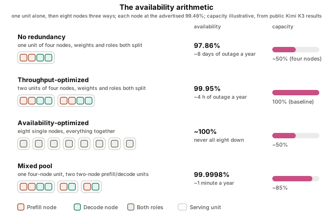
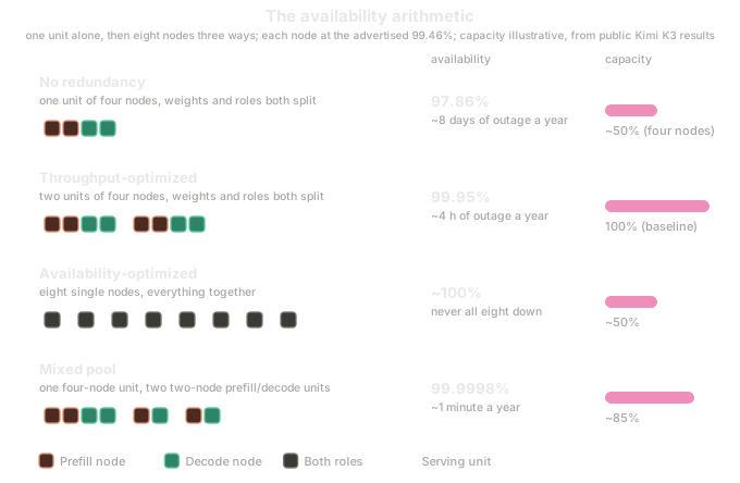
Availability compounds against you: four respectable nodes alone make a 97.86% service, almost eight days of outage a year. Shape buys it back: the mixed pool keeps about 85% of peak capacity and brings that down to about a minute.

Even the failover is different here. Agentic routing is not a reverse proxy spreading load: it is saturation-aware and, above all, KV-cache aware, because a session’s context lives where the session was served. Requests that land on a fresh unit pay full prefill on hundred-thousand-token contexts, so while a failed unit restores, time-to-first-token and per-user speed sag before they recover. That sag is part of the price of availability too.

A provider claiming the lowest theoretical token cost by running every GPU at permanent saturation is not necessarily operating the cheapest reliable service; it may just be one incident away from proving the difference. And availability itself has a price curve: 99%, 99.9% and 99.99% are not the same machine count, so they are not the same token cost. When you compare providers, you are comparing SLOs whether anyone says so or not.

6. Just the beginning

Serving trillions of tokens each month has taught us a lot, and DeepSeek V4 Flash is one place where that learning shows. We have served it faster than anyone since the day the weights were released, the model’s own published fleet included; and for agentic serving, the delivered-token frontier above is the highest documented anywhere. The same discipline runs across our lineup: every model’s frontier is validated in the lab first, and production then runs the shape its demand pays for.

We are proud of the stages behind us, and this is the beginning. Demand for tokens is growing at a pace the world’s compute supply will strain to meet, and that tension will test everyone in the chain, inference providers first. Efficiency is how the equation closes, so we keep doing our part: obsessing over the question we opened with, the highest-value automated work at the lowest cost, and challenging our own excellence with a community that never lets us settle.

References

• Rethinking AI factory economics. NVIDIA on cost per token as the metric that matters, and the basic formula.
• DSpark: load-aware speculative decoding. DeepSeek’s published production frontier for V4 Flash, and the MTP and DSpark baseline curves above.
• DeepSeek-V4 technical report. The compressed-attention architecture, and the FLOPs and KV reductions quoted in section 4.
• Artificial Analysis: DeepSeek V4 Flash providers. Provider-level retail price and per-request speed, the two public numbers that are not production cost.
• NVIDIA AI inference. The 5x software-only token cost improvement on B200 cited in section 4.
• SGLang and vLLM. The open-source serving engines this class of engineering builds on.
• InferenceX. SemiAnalysis’s continuous, open benchmark of inference hardware and engines. We are fans, and the Kimi K3 charts above are drawn from its published data (Apache 2.0).
• DeepSeek V4 Pro DSpark: the model isn’t ready, the architecture is. Our deep dive on this architecture and on DSpark, and the maturity lesson in section 4.